Monodromy Matrix Analysis for Power Converters

1What is Monodromy?

A switching converter is a periodically-switched dynamical system. Every switching period $T = 1/f_s$, the circuit topology changes: a transistor turns on, current flows through one path, then the transistor turns off and current takes another. The state vector $\mathbf{x} = [i_L,\; v_C]^\top$ evolves continuously within each sub-interval but experiences an abrupt change in its governing equation at each switching instant.

The standard approach — state-space averaging — smooths out this periodicity by averaging the on-state and off-state dynamics over one period. The result is a continuous, time-invariant model that supports classical frequency-domain design (Bode plots, phase margin, gain margin). This works well when the control bandwidth $f_c$ is much smaller than $f_s$.

Monodromy analysis takes a different path. Instead of averaging away the switching, it embraces the periodicity and asks a precise question:

If I perturb the converter's state by a small amount $\delta\mathbf{x}$ at the beginning of a switching period, what is the perturbation $\delta\mathbf{x}'$ one full period later?

The answer is a linear map:

$$\delta\mathbf{x}(nT + T) = M \cdot \delta\mathbf{x}(nT)$$

The matrix $M$ is the monodromy matrix (also called the Floquet multiplier matrix or state transition matrix over one period). Its eigenvalues $\lambda_i$ are the Floquet multipliers. Stability is determined by a simple rule:

Stability criterion: The periodic orbit is stable if and only if all eigenvalues of $M$ satisfy $|\lambda_i| < 1$ (all lie inside the unit circle in the complex plane).

For a buck converter with PI control, the state vector is $\mathbf{x} = [i_L,\; v_C,\; \xi]^\top$ where $\xi$ is the integrator state. In each sub-interval, the dynamics are linear:

$$\dot{\mathbf{x}} = A\mathbf{x} + \mathbf{b}_k, \qquad k \in \{\text{on},\; \text{off}\}$$

The state transition through each sub-interval is the matrix exponential $e^{A \cdot \Delta t}$. But there is a subtlety at the switching instant itself — a perturbation shifts the timing of the switch, not just the state. This is captured by the saltation matrix.

Four-panel monodromy analysis of a buck converter: max|λ| vs Kp, max|λ| vs Ki, eigenvalue locus on the unit circle, and 2-D stability map in the Kp-Ki plane. — **Fig. 1.** Monodromy overview for a VM-PI buck converter. (a) max$|\lambda|$ vs $K_p$; (b) max$|\lambda|$ vs $K_i$ showing the critical value $K_{i,\text{crit}} = 189$; (c) eigenvalue locus migrating toward the unit circle; (d) stability map in the $K_p$–$K_i$ plane (colour = max$|\lambda|$).

2The Saltation Matrix

The switching instant is defined by a switching surface $h(\mathbf{x}, t) = 0$. For voltage-mode PWM with a PI controller:

$$h(\mathbf{x}, t) = K_p(V_\text{ref} - v_C) + K_i\xi - v_\text{ramp}(t)$$

When the control signal $u(t)$ crosses the sawtooth ramp, the switch turns off. A perturbation $\delta\mathbf{x}$ at the switching instant causes two effects:

The state itself is perturbed: the converter is at a slightly different $\mathbf{x}$.
The switching time shifts by $\delta t$, because the perturbed state crosses the switching surface at a different moment.

The saltation matrix $S$ accounts for both effects simultaneously:

$$S = I + \frac{(\mathbf{f}^+ - \mathbf{f}^-)\,\mathbf{n}_h^\top} {\mathbf{n}_h^\top \mathbf{f}^- - \partial h / \partial t}$$

where:

$\mathbf{f}^-$ and $\mathbf{f}^+$ are the vector fields just before and after the switch,
$\mathbf{n}_h^\top = \partial h / \partial \mathbf{x}$ is the normal to the switching surface,
$\partial h / \partial t = -S_e$ is the ramp slope.

For the buck converter, $A_\text{on} = A_\text{off}$ (the state matrix is the same in both sub-intervals — only the input voltage source switches). So:

$$\mathbf{f}^+ - \mathbf{f}^- = \mathbf{b}_\text{off} - \mathbf{b}_\text{on} = \begin{bmatrix} -V_\text{in}/L \\ 0 \\ 0 \end{bmatrix}$$

This is a constant vector — independent of the operating point. The full monodromy matrix is then:

$$M = e^{A(1-D)T}\; S\; e^{ADT}$$

For the boost converter, $A_\text{on} \neq A_\text{off}$ (the inductor-capacitor coupling changes with the switch state), so:

$$\mathbf{f}^+ - \mathbf{f}^- = (A_\text{off} - A_\text{on})\mathbf{x}^* + (\mathbf{b}_\text{off} - \mathbf{b}_\text{on}) = \begin{bmatrix} -v_C^*/L \\ i_L^*/C \\ 0 \end{bmatrix}$$

This depends on the operating point $\mathbf{x}^*$ at the switching instant. The saltation is state-dependent: both the current and voltage perturbations feed into different rows of $S$, coupling the two state variables through the switching event.

3Buck Converter: Monodromy vs Phase Margin

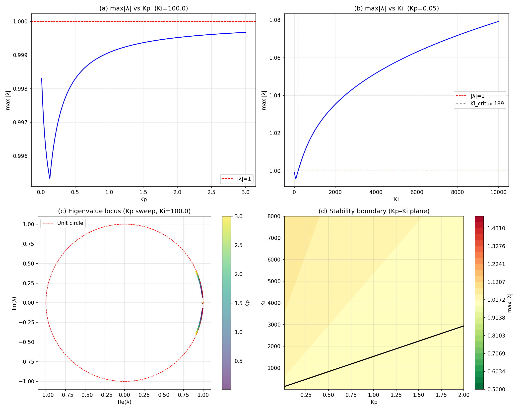
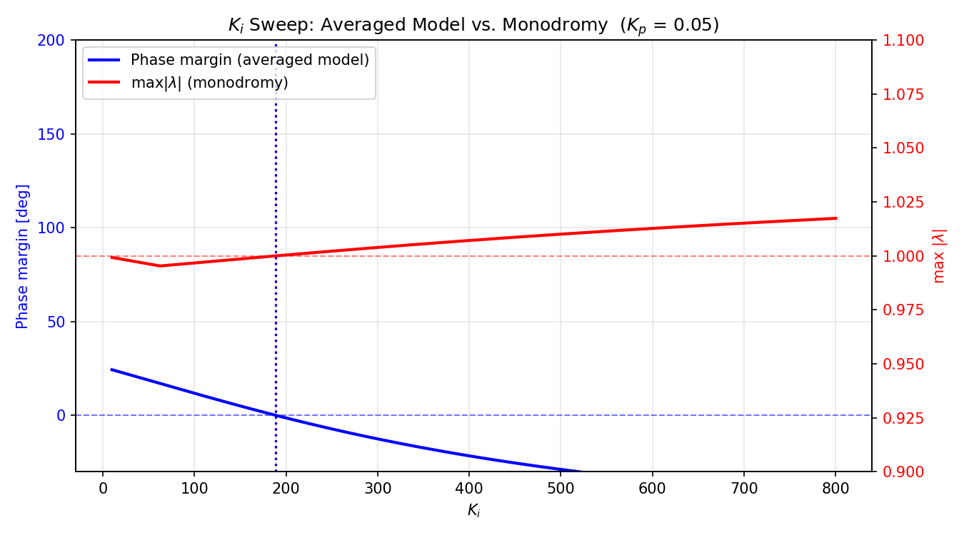
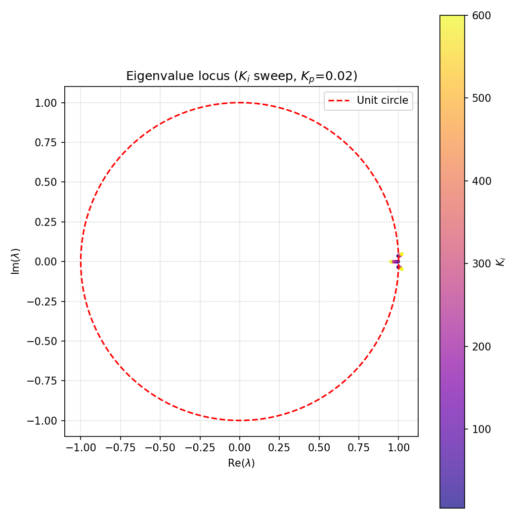
The first test: a VM-PI controlled buck converter ($V_\text{in} = 12$ V, $V_\text{ref} = 5$ V, $L = 100\;\mu$H, $C = 220\;\mu$F, $R = 5\;\Omega$, $f_s = 100$ kHz). Fix $K_p = 0.05$ and sweep $K_i$ from 0 to 600.

The averaged model predicts instability (PM $= 0$) at a critical $K_i$. The monodromy matrix predicts instability ($\max|\lambda| = 1$) at the same critical $K_i$.

Result: Both methods agree. The critical $K_i$ values match to within 0.1%. The instability is a Neimark–Sacker bifurcation: the dominant eigenvalue pair exits the unit circle at an angle near $0°$ (corresponding to the LC resonance frequency $f_0 \approx 34$ Hz, far below $f_s$).

Ki sweep comparing phase margin (blue) and monodromy spectral radius (red) for a buck converter. Both cross the stability boundary at the same Ki. — **Fig. 2.** $K_i$ sweep ($K_p = 0.05$): phase margin (blue, left axis) and max$|\lambda|$ (red, right axis). Both methods cross the stability boundary at $K_i \approx 189$.

Switched ODE Validation

To confirm that the monodromy prediction is not just a mathematical coincidence, we run the exact switched ODE: solve the circuit differential equation cycle by cycle, detecting the switching instant via event detection (control signal crosses the ramp).

The state is sampled stroboscopically at $t = nT$ (once per switching period). A small perturbation is applied, and its norm $\|\delta\mathbf{x}(nT)\|$ is tracked over 200 cycles. The measured decay/growth rate is compared to the predicted rate $\max|\lambda|$.

Case	$K_i$	PM	$\max\|\lambda\|$	Measured rate	Verdict
Stable	100	11.8°	0.9967	≈ 0.997	Agree
Critical	≈ 189	0°	1.000	≈ 1.000	Agree
Unstable	600	−34.6°	1.013	1.014	Agree

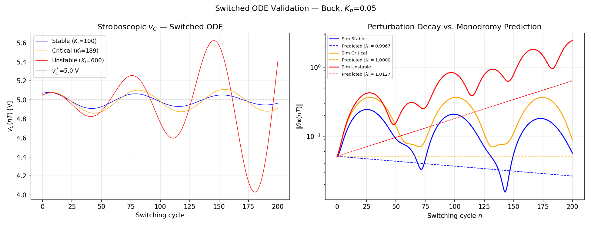
Switched ODE validation: stroboscopic vC traces for stable, critical, and unstable Ki, plus perturbation decay/growth vs monodromy prediction. — **Fig. 3.** Switched ODE validation. Left: stroboscopic $v_C(nT)$ for stable ($K_i = 100$, blue), critical ($K_i = 189$, orange), and unstable ($K_i = 600$, red) cases. Right: perturbation norm (solid) vs monodromy prediction (dashed). The unstable case's measured growth rate of 1.014 matches the predicted 1.013.

The unstable case grows at 1.4% per cycle — the simulation diverges exactly as the monodromy predicts. But both methods see this instability. There is no disagreement yet, because the instability is slow-scale.

4Boost Converter: The RHP Zero

The boost converter ($V_\text{in} = 5$ V, $V_\text{ref} = 12$ V, $D = 0.583$) introduces two complications not present in the buck:

Topology-dependent matrices. $A_\text{on} \neq A_\text{off}$ — the inductor-capacitor coupling disappears when the switch is on (the diode is reverse-biased).
Right-half-plane (RHP) zero. The averaged plant $G_{vd}(s)$ has a zero in the right half plane at $\omega_z = (1-D)^2 R / L$. This limits achievable bandwidth and causes rapid phase deterioration.

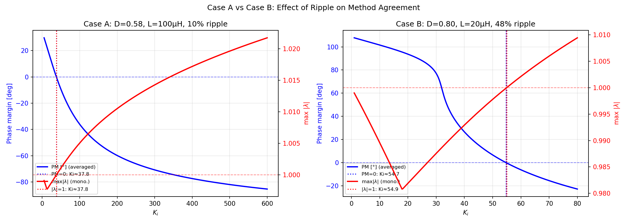
Do these complications cause the two methods to disagree? We sweep $K_i$ for two cases:

Case	$D$	Ripple	$K_{i,\text{crit}}$ (monodromy)	$K_{i,\text{crit}}$ (averaged)
Moderate step-up	0.583	10%	37.8	37.8
High step-up	0.800	48%	54.9	54.7

Result: The two methods agree to within $\Delta K_i < 0.2$ even at 48% inductor current ripple.

Ki sweep for boost converter Case A (10% ripple) and Case B (48% ripple). Phase margin and monodromy spectral radius cross the stability boundary at nearly identical Ki in both cases. — **Fig. 4.** Boost converter $K_i$ sweeps. Case A ($D = 0.58$, 10% ripple, left) and Case B ($D = 0.80$, 48% ripple, right). Blue: phase margin; red: max$|\lambda|$. The stability boundaries nearly coincide in both cases.

Why Do They Still Agree?

The RHP zero is not a modeling artifact of averaging — it is a real physical phenomenon. When the duty cycle increases, the switch is on longer, blocking the inductor current from reaching the output. The capacitor current drops immediately. Both the averaged model and the monodromy encode this same physics.

And the instability mechanism is still Neimark–Sacker: the eigenvalue pair exits the unit circle at an angle corresponding to the LC resonance, far below $f_s$. Since this is a slow-scale phenomenon, the averaged model captures it correctly.

But the monodromy reveals something the averaged model does not: the saltation is state-dependent and bidirectional. A voltage perturbation affects the current dynamics and vice versa. This structural richness becomes important when the operating point is extreme or the control bandwidth is pushed high.

Eigenvalue locus for the boost converter as Ki is swept. The complex pair migrates outward toward the unit circle, confirming a Neimark-Sacker bifurcation. — **Fig. 5.** Boost eigenvalue locus ($K_p = 0.02$, $K_i$ swept). The complex pair migrates outward and exits the unit circle, confirming a Neimark–Sacker bifurcation identical in character to the buck.

5Where the Averaged Model Breaks Down

The Averaging Assumption

State-space averaging replaces the switched forcing

$$\mathbf{b}(t) = \begin{cases} \mathbf{b}_\text{on} & 0 \le t - nT < d\,T \\ \mathbf{b}_\text{off} & d\,T \le t - nT < T \end{cases}$$

with its period-average:

$$\bar{\mathbf{b}}(t) = d(t)\,\mathbf{b}_\text{on} + \bigl(1 - d(t)\bigr)\,\mathbf{b}_\text{off}$$

This is exact when $d(t)$ is constant over each period. It is an approximation otherwise, with error proportional to $\Delta d = d(nT + T) - d(nT)$.

When $f_c \ll f_s$, the duty cycle changes slowly: $\Delta d \approx 0$ per period, and averaging is accurate.

When $f_c \to f_s$, the high-gain control drives the duty cycle to change significantly within a single period. The "averaged $d$" no longer represents what the circuit actually sees cycle by cycle.

Experiment: High-Bandwidth Buck

To make this visible, we use a buck converter with a small output capacitor $C = 10\;\mu$F (LC resonance $f_0 \approx 5$ kHz, vs $f_s = 100$ kHz). Fix $K_i = 100$ and sweep $K_p$ from 0.01 to 5, pushing the crossover frequency $f_c$ from a few kHz toward $f_s/3$.

$K_p$	$f_c$ [kHz]	$f_c / f_s$	PM	$\max\|\lambda\|$	$\angle\lambda$	Type
0.30	10.5	10.5%	21.8°	0.997	0°	Neimark–Sacker
1.00	19.5	19.5%	11.5°	0.999	0°	Neimark–Sacker
3.00	30.7	30.7%	6.2°	1.000	0°	Neimark–Sacker
4.00	35.3	35.3%	5.4°	2.203	180°	Period-2
5.00	39.2	39.2%	4.8°	3.788	180°	Period-2

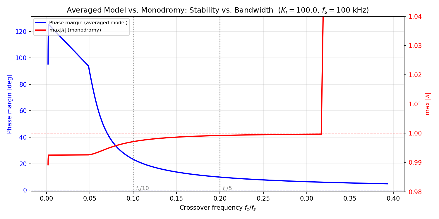
Phase margin and monodromy spectral radius vs normalised bandwidth fc/fs. The monodromy spectral radius spikes above 1.0 at fc/fs ≈ 0.32 while phase margin stays positive, creating a disagreement zone. — **Fig. 6.** Stability vs bandwidth ($K_i = 100$, $K_p$ swept). Blue: phase margin (left axis); red: max$|\lambda|$ (right axis). The shaded region marks where monodromy predicts instability but the averaged model reports positive PM. The averaged model never crosses PM $= 0$.

A dramatic transition happens at $K_p \approx 3.24$ ($f_c \approx 31.7$ kHz = 31.7% of $f_s$):

Below: the dominant eigenvalue is near angle $0°$ and slowly approaching $|\lambda| = 1$ (Neimark–Sacker). Both methods agree.
Above: the dominant eigenvalue jumps to angle $180°$ and $|\lambda| \gg 1$. This is a period-doubling bifurcation. The averaged model still reports positive phase margin.

Monodromy: $K_{p,\text{crit}} = 3.24$, instability at $f_c = 31.7$ kHz (31.7% $f_s$).

Averaged model: No instability found. PM stays positive across the entire sweep.

Why the Averaged Model Is Blind

A period-doubling instability is an alternating-cycle pattern: the perturbation flips sign every period, repeating every two periods. Its frequency is $f_s/2$ — the Nyquist frequency of the stroboscopic map.

When the averaged model integrates over one period, it folds the $f_s/2$ component to DC and discards it. The resulting continuous transfer function $G_{vd}(s)$ has no poles or zeros at $f_s/2$. It cannot see the instability because the instability exists at a frequency that averaging, by construction, eliminates.

The physical mechanism is the saltation entry $S_{12}$, which maps a voltage perturbation $\delta v_C$ into a current correction $\delta i_L$ at each switching instant. $S_{12}$ grows linearly with $K_p$. When it is large enough, the alternate-cycle correction exceeds the original perturbation: the eigenvalue at $180°$ exits the unit circle.

Switched ODE Confirmation

Three operating points are validated with the exact switched ODE:

Case	$K_p$	$f_c/f_s$	PM	$\max\|\lambda\|$	Simulation
Low BW	0.30	10.5%	21.8°	0.997	Stable (confirmed)
Mid BW	3.08	30.9%	6.2°	1.000	Stable (confirmed)
High BW	3.88	34.7%	5.5°	2.015	Diverges in ∼30 cycles

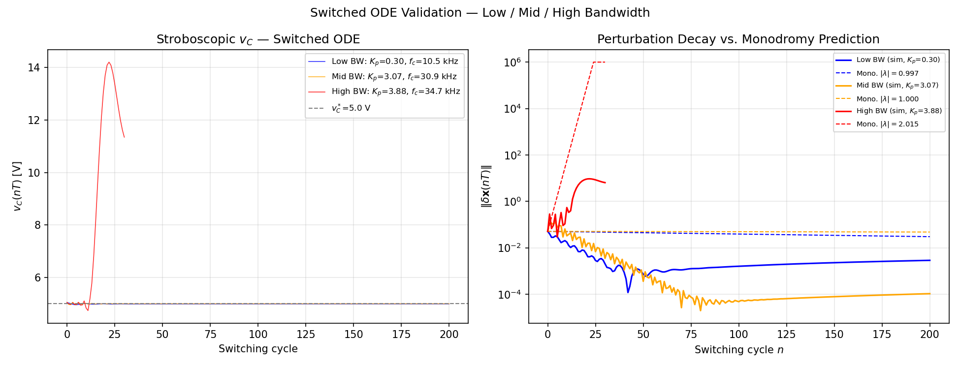
Switched ODE validation at three bandwidth points: low BW (stable), mid BW (stable), and high BW (diverges within ~30 cycles). Perturbation decay plot shows monodromy predictions matching simulation. — **Fig. 7.** Switched ODE validation at three bandwidths. Left: stroboscopic $v_C(nT)$ — the high-BW case (red) diverges rapidly while the averaged model predicts PM $= 5.5°$. Right: perturbation norm vs monodromy prediction (dashed). The high-BW measured growth confirms the monodromy eigenvalue.

The high-bandwidth case diverges within approximately 30 switching cycles, confirming the monodromy prediction. The averaged model's positive phase margin of 5.5° is simply wrong.

Practical Design Rule

$f_c < f_s/10$: Use the averaged model freely. Both methods agree.
$f_c \in [f_s/10,\; f_s/3]$: The averaged model may be unsafe. Monodromy or discrete-time analysis is required.
$f_c > f_s/3$: The averaged model is unreliable. Period-doubling is likely.